How to Fix Google Sheets 'FILTER Has Mismatched Range Sizes' (#VALUE!)

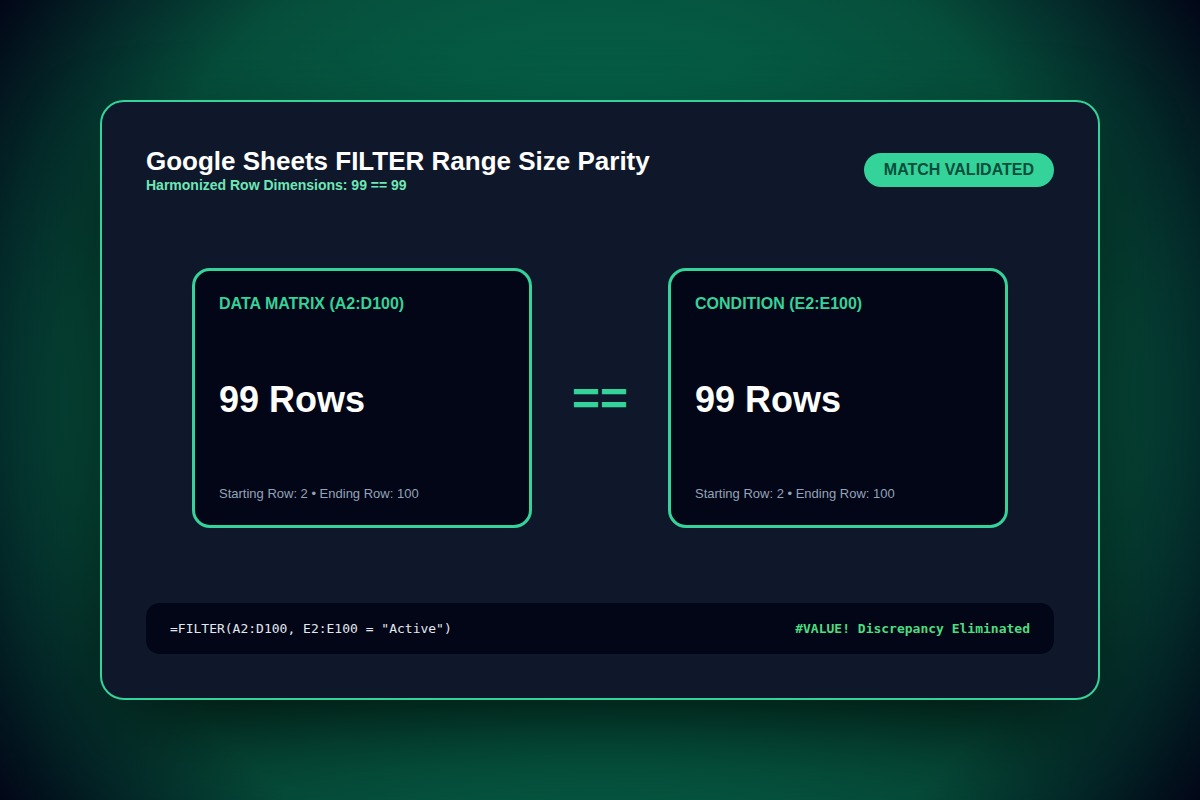
Harmonize the start and end row numbers of your source range and all condition arguments. E.g., change =FILTER(A2:C100, D2:D50 = 'Won') to =FILTER(A2:C100, D2:D100 = 'Won').
=FILTER(A2:C100, D2:D100 = "Won")Why Does This Error Happen?
The FILTER function executes row-by-row boolean masking. When the condition array has fewer or more rows than the target dataset, the index vectors do not match, triggering a fatal #VALUE! exception.
Step-by-Step Diagnostic & Resolution Walkthrough
1Step 1: Check Row Indices Across All Condition Arguments
Examine every boolean argument separated by commas. Verify that if the source range starts at row 2 and ends at row 500, every filter condition also starts at 2 and ends at 500.
=FILTER(A2:D500, (B2:B500 = "Paid") * (C2:C500 > 100))2Step 2: Use Open-Ended Ranges Safely
If using dynamic open ranges like A2:A, ensure your condition also uses open ranges like B2:B, rather than a hardcoded boundary like B2:B200.
=FILTER(A2:D, B2:B = "In Progress", C2:C <> "")3Step 3: Wrap in IFERROR or FILTER Guard
Prevent formula errors when no matching records satisfy all conditions by passing an optional empty return value or wrapping with IFERROR.
=IFERROR(FILTER(A2:D100, E2:E100 = "Approved"), "No matching records")Troubleshooting Matrix & Configuration Rules
| Formula Syntax | Evaluation Result | Status |
|---|---|---|
| =FILTER(A2:C100, D2:D100 = 'Yes') | 100 rows vs 100 rows | Valid (Executes Cleanly) |
| =FILTER(A2:C100, D2:D50 = 'Yes') | 100 rows vs 50 rows | Error (#VALUE! Mismatched sizes) |
| =FILTER(A2:C, D2:D = 'Yes') | Open range vs Open range | Valid (Auto-expands to sheet bottom) |
← Swipe horizontally to view full table →
Still Not Working? Check These Edge Cases
Fix: When filtering horizontally across columns (e.g. A1:Z1), condition arrays must match column width (e.g. A2:Z2), not vertical row height.
Frequently Asked Questions
Can I combine OR logic inside Google Sheets FILTER?
Yes, use the addition operator (+) for OR conditions: =FILTER(A2:C100, (D2:D100 = 'Active') + (D2:D100 = 'Pending')). Use the multiplication operator (*) for AND conditions.