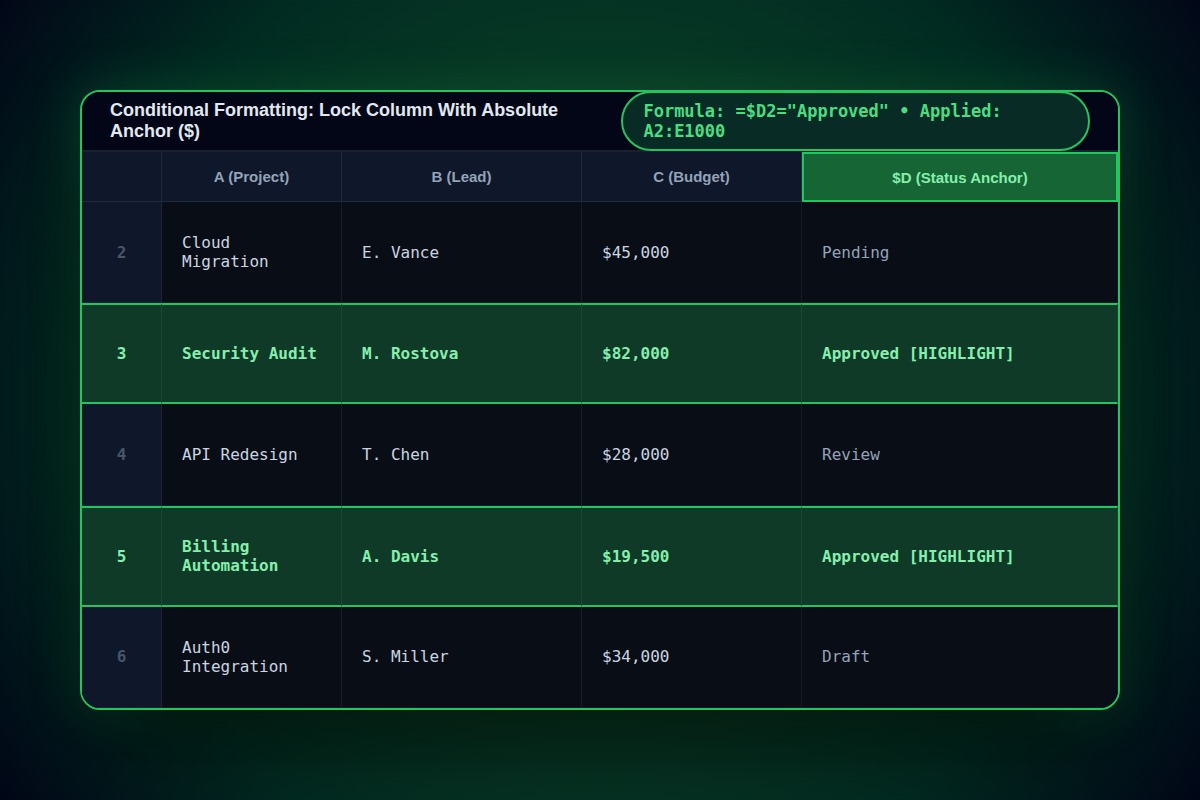
How to Highlight Entire Row in Google Sheets Conditional Formatting

In Conditional Formatting > Custom Formula, add a dollar sign ($) before the column letter to lock evaluation to that specific column across all cells in the row: =$C2="Approved". Apply the rule to the entire sheet range (A2:Z1000).
=$C2="Approved"Why Does This Error Happen?
Without the dollar sign ($) anchor, Google Sheets applies relative cell referencing. Each column shifts the check to its adjacent column, resulting in single-cell highlights or staggered formatting.
Step-by-Step Diagnostic & Resolution Walkthrough
1Step 1: Select the Full Target Data Range
Highlight all rows you want formatted (e.g. A2:Z100). Do not include header row 1.
2Step 2: Set Format Rules to 'Custom Formula is'
Open Format > Conditional Formatting. In the 'Format cells if' dropdown, scroll down and choose 'Custom formula is'.
3Step 3: Enter Formula with Column Lock ($)
Precede the target column with a dollar sign. Ensure the row number matches the first row in your 'Apply to range'.
=$D2=TRUETroubleshooting Matrix & Configuration Rules
| Formula Syntax | Behavior Across Row | Intended Use Case |
|---|---|---|
| =C2="Done" | Highlights only column C cell | Individual cell alert |
| =$C2="Done" | Highlights entire row A through Z | Full row status indicator |
| =$C$2="Done" | Highlights entire sheet based on C2 | Global toggle rule |
← Swipe horizontally to view full table →
Still Not Working? Check These Edge Cases
Fix: Mismatch between range start and formula row causes a 1-row offset. Always synchronize row numbers (e.g. Range A2:Z with Formula =$C2).
Frequently Asked Questions
How do I highlight a row when a checkbox is checked?
If checkboxes are in column E, use the formula: =$E2=TRUE.